

|
CGAL 5.0 - K Discrete Oriented Polytope Tree (K-DOP Tree)
|
|
CGAL 5.0 - K Discrete Oriented Polytope Tree (K-DOP Tree)
|
The KDOP_tree package offers a data structure and algorithms for efficient ray and distance queries on 3D triangular meshes using k-DOPs. The algorithms include intersection detection, intersection computation and distance computation. Currently all the intersection algorithms are available for ray queries, and the distance computation includes algorithms to compute the closest point on the primitives from the point query.
The K-DOP tree data structure is implemented based on the existing AABB tree data structure, which takes an iterator range of geometric data as input and converts into primitives. A hierarchy of k-DOPs is constructed by first splitting the primitives in the same way as in AABB tree, i.e. a binary tree splitting along the longest axis, and then computing k-DOPs of each primitive and each node in a recursive bottom-top manner.
The main function interface is in class KDOP_tree which creates the k-DOP tree from an iterator range of geometric data. Once a k-DOP tree has been built, the algorithms for ray and distance queries can be applied. The interface functions share the same name with those defined in class AABB_tree.
^^
A k-DOP is a bounding volume that is determined by a fixed \(k\) ( \(k \geq 6\) in 3D) directions \(\{\boldsymbol{d}_1, \cdots, \boldsymbol{d}_{k/2}, \boldsymbol{d}_{k/2 + 1}, \cdots, \boldsymbol{d}_k\}\) [2]. In the implementation, the first \(k/2\) directions are given which should not be colinear between each other. For each direction \(\boldsymbol{d}_i (i = 1, \cdots, k/2)\), there is always an opposite direction \(\boldsymbol{d}_{k/2 + i}\).
In each direction \(\boldsymbol{d}_i\), a support height \(h_i\) is computed as the maximum projected value of the primitive set on the direction, i.e. \(h_i = \max_j(\boldsymbol{x}_j \cdot \boldsymbol{d}_i)\) where \(\boldsymbol{x}_j\) are coordinates of vertices in the set of primitives. In the implementation, a k-DOP is represented as \(k\) support heights in \(k\) directions. If unit directions (that is, the norm of the direction vector is 1) are considered to construct the k-DOP, each direction \(\boldsymbol{d}_i\) together with its corresponding support height \(h_i\) represent a half plane, and the \(k\) half planes bound the object. Note that it is not necessary to take unit directions to construct the k-DOP for the query purposes.
An AABB can be seen as a 6-DOP with six unit directions in \(\pm x\), \(\pm y\) and \(\pm z\) axes. Compared with the AABB, the k-DOP with \(k > 6\) can provide a tighter bound for the object.
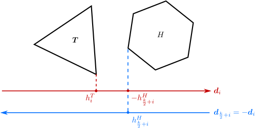
For checking the overlap between two k-DOPs of mesh objects, it is straightforward to compare support heights (representing the k-DOPs) of the two objects in \(k\) directions. As illustrated in Figure fig__figkdop_overlap, the triangle object and the hexagon object do not overlap in the direction \(\boldsymbol{d}_i\), if
\(h_i^T < -h_{k/2 + i}^H\), that is, \(h_i^T + h_{k/2 + i}^H < 0\).
The algorithm of overlap detection between two k-DOPs is implemented in the function KDOP_kdop::do_overlap_kdop.
^^
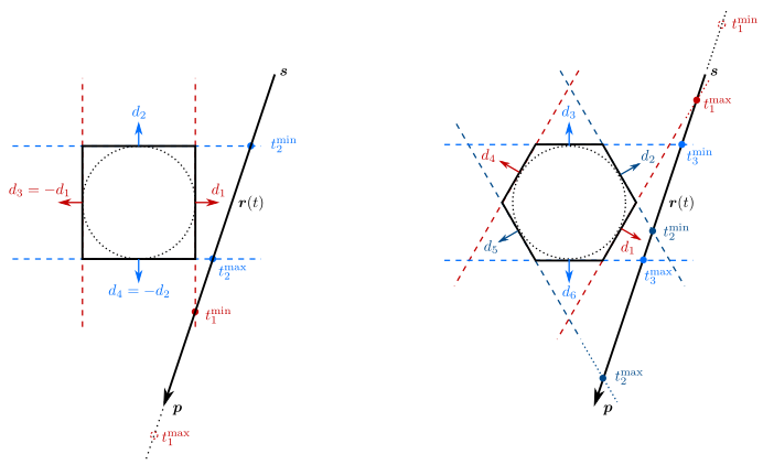
For an efficient ray/k-DOP overlap detection, the intersections between the ray and parallel slabs (corresponding to opposite directions \(\boldsymbol{d}_i\) and \(\boldsymbol{d}_{k/2 + i}\)) are considered [1], as shown in Figure fig__figkdop_ray.
In each direction \(\boldsymbol{d}_i\), there is a plane equation at the vertex where the support height \(h_i\) is evaluated,
\[ \boldsymbol{d}_i \cdot \boldsymbol{x} - h_i = 0 \, . \]
Substituting the ray equation \( \boldsymbol{r}(t) = (\boldsymbol{p} - \boldsymbol{s})t + \boldsymbol{s} \) into the plane equation yields,
\[ t_i = \frac{h_i - \boldsymbol{d}_i\cdot\boldsymbol{s}}{\boldsymbol{d}_i\cdot\boldsymbol{p} - \boldsymbol{d}_i\cdot\boldsymbol{s}} = \frac{h_i - h_i^s}{h_i^p - h_i^s} \, , \]
where \(h_i\) is the support height of the primitives in the direction \(\boldsymbol{d}_i\), \(h_i^s\) and \(h_i^p\) are the projected value of the source point \(\boldsymbol{s}\) and the second point \(\boldsymbol{p}\) of the ray on the direction \(\boldsymbol{d}_i\). There are two intersection parameters \(t\) between the ray and two parallel slabs in each direction, and \(t_i^{\min}\) and \(t_i^{\max}\) depend on the ray direction and the k-DOP direction (merely comparing \(h_i^s\) and \(h_i^p\)). Note that the special case \(h_i^s = h_i^p\) (i.e. the ray is parallel to the slabs) should be treated separately.
The ray and the k-DOP do not overlap if there exists a direction \(\boldsymbol{d}_i\) whose intersection parameter range \([t_i^\min, t_i^\max]\) does not overlap with the range \([t_j^\min, t_j^\max]\) in any other direction \(\boldsymbol{d}_j\). In the implementation, \(t^\min\) is updated with the larger \(t_j^\min\), and \(t^\max\) is updated with the smaller \(t_j^\max\). As long as \(t^\min > t^\max\), the ray and the k-DOP are detected as not overlapping.
The algorithm of overlap detection between a ray and a k-DOP is implemented in the function KDOP_kdop::do_overlap_ray.
^^
The following example shows the computation of first intersection between a ray and a triangular mesh, that is, the intersection point closest to the source of the ray. Without explicitly given, the directions of k-DOPs are pre-defined according to the prescribed number of directions NUM_DIRECTIONS. For \(k = 14\), the pre-defined directions are \((1, 0, 0), (0, 1, 0), (0, 0, 1), (1, 1, 1), (-1, 1, 1), (-1, -1, 1), (1, -1, 1)\) and their opposites (i.e. directions corresponding to axes and body diagonals).
File KDOP_tree/kdop_ray_query.cpp
In the following example the closest point in the set of primitives between a point and the triangular mesh is computed. The pre-defined directions ared used for computing the k-DOPs.
File KDOP_tree/kdop_distance_query.cpp
The following example shows how to visualise the k-DOPs, since the k-DOPs are represented as support heights in the implementation. In the example, we show how to define and set user-defined directions for k-DOPs instead of using default directions. The number of user-defined directions must be the same as NUM_DIRECTIONS. A half plane can then be created with a direction and the associated support height. The intersections of all half planes form a convex hull which visualises the k-DOP.
Note that unit direction vectors should be used for the visualisation. Nonetheless, this is not a restriction for the users as internally all user-defined directions are automatically converted into unit vectors in the implementation.
File KDOP_tree/kdop_polytopes.cpp
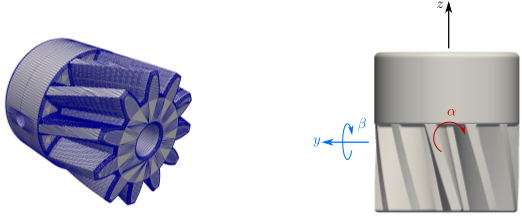
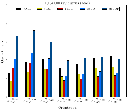
The performance of the k-DOP tree is demonstrated with an example of a gear with a skewed mesh as shown in Figure fig__fig_kdop_gear. The gear mesh contains 28,346 vertices and 56,700 triangles. We consider two parameters as variables: the rotation angle \(\alpha\) about \(+x\) axis and the rotation angle \(\beta\) about \(+y\) axis. The influence of variations of the two variables (i.e. orientations of the gear) on the performance will be examined.
^^
As \(k\) increases, the build time for the k-DOP tree also increases slightly. Meanwhile, the time for a 6-DOP is slightly more than the equivalent AABB. The reason for this is that the splitting process follows the AABB tree which also computes the bounding boxes of each node.
| Schemes | AABB | 6-DOP | 14-DOP | 18-DOP | 26-DOP |
|---|---|---|---|---|---|
| Built time (s) | 0.0354 | 0.039 | 0.0426 | 0.0455 | 0.0493 |
The k-DOP gives a tighter bound than AABB, and the bounding volume is tighter with a higher \(k\). We take the gear mesh with \(\alpha = \pi/4\) and \(\beta = \pi/4\) as an example. The following table shows the number of nodes traversed and the number of primitives traversed in the tree to get all intersections with 1,134,000 rays. As it is indicated in the table, the number of nodes and primitives visited in the tree are reduced significantly as \(k\) increases. The similar result can be observed considering other orientations of the gear mesh.
| Schemes | AABB | 6-DOP | 14-DOP | 18-DOP | 26-DOP |
|---|---|---|---|---|---|
| No. of nodes traversed | 675,121,081 | 675,121,081 | 380,445,767 | 328,388,685 | 292,286,940 |
| No. of leaves traversed | 168,794,139 | 168,794,139 | 73,849,181 | 53,532,425 | 42,911,934 |
The query time for ray intersections depends on the orientations of the mesh. We take the gear mesh with \(\alpha = \pi/4\) and \(\beta = \pi/4\) as an example.The following table compares the ray query time with AABB and different k-DOPs. As can be seen from the table, the ray query time reduces when using k-DOP with \(k > 6\).
| Functions | AABB | 6-DOP | 14-DOP | 18-DOP | 26-DOP |
|---|---|---|---|---|---|
KDOP_tree::do_intersect() | 5.5 | 4.596 | 4.14 | 4.44 | 5.128 |
KDOP_tree::any_intersection() | 5.156 | 4.428 | 4.128 | 4.276 | 5.052 |
KDOP_tree::first_intersection() | 11.576 | 11.708 | 9.152 | 8.836 | 9.916 |
KDOP_tree::all_intersections() | 25.472 | 22.656 | 19.664 | 19.348 | 21.908 |
To demonstrate the influence of orientations of the mesh on the query time, we consider seven different orientations and plot the query time of KDOP_tree::do_intersect. When the mesh is axis-aligned, i.e. \(\alpha = 0\) and \(\beta = 0\), 6-DOP takes the least query time, even compared with the equivalent AABB tree. The k-DOP (e.g. \(k = 14\) and \(k = 18\)) tree takes less time when the mesh is not axis-aligned.
^^
In addition, 26-DOP consumes more time than 14-DOP and 18-DOP in this example, and this is because the number of operations in the overlap check increases with a larger \(k\) while the number of nodes and primitives traversed in the tree are reduced. The trade-off between the increased number of operations proportional to \(k\) and the reduced number of overlap checks can influence the performance of the k-DOP tree.
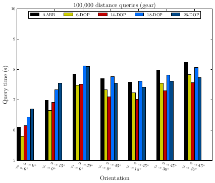
To compare the distance query time, we consider 100,000 random points and compute their closest points in the mesh, and different orientations of the mesh are also considered. The result is shown in Figure fig__fig_kdop_distance_query_gear. It can be observed that the k-DOP ( \(k > 6\)) is faster than AABB tree when the mesh is not axis-aligned, and the 6-DOP is faster than the equivalent AABB tree.
^^
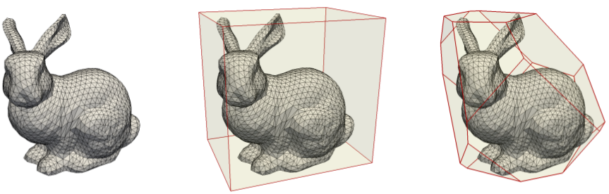
In general, the k-DOP is more efficient than the AABB when there is a larger portion of skewed triangles in the mesh. However, it has to be mentioned that with tests on several isotropic meshes (e.g. the bunny mesh in Figure fig__figkdop_bunny), the k-DOP tree is not as efficient as the AABB tree structure for ray and distance queries. We think it is related to the trade-off between the increased number of operations (due to increased \(k\)) and the reduced number of overlap checks.
As an example of the istropic mesh, the bunny mesh fig__figkdop_bunny is subdivided four times with a Loop subdivision method. The refined mesh contains 132,546 vertices and 265,088 triangles. We considered 5,301,760 random rays and 100,000 random points. The results of ray and distance queries are shown in the following table. The AABB tree is more efficient than the k-DOP tree ( \(k > 6\)).
| Functions | AABB | 6-DOP | 14-DOP | 18-DOP | 26-DOP |
|---|---|---|---|---|---|
KDOP_tree::build() | 0.184 | 0.208 | 0.224 | 0.236 | 0.268 |
KDOP_tree::do_intersect() | 7.996 | 7.264 | 10.6 | 12.496 | 15.748 |
KDOP_tree::any_intersection() | 7.692 | 7.160 | 10.268 | 12.08 | 15.436 |
KDOP_tree::first_intersection() | 17.856 | 18.264 | 20.94 | 23.912 | 28.804 |
KDOP_tree::all_intersections() | 36.188 | 31.984 | 36.272 | 40.624 | 49.496 |
KDOP_tree::closest_point() | 22.256 | 21.816 | 24.94 | 25.588 | 27.428 |
This package was developed by Xiao Xiao as a project of the Google Summer of Code 2019, mentored by Fehmi Cirak and Andreas Fabri. It is inspired from a version that was developed at the University of Cambridge by Xiao Xiao.
 1.8.11